Turning Pixels Into Something the AI Can Eat

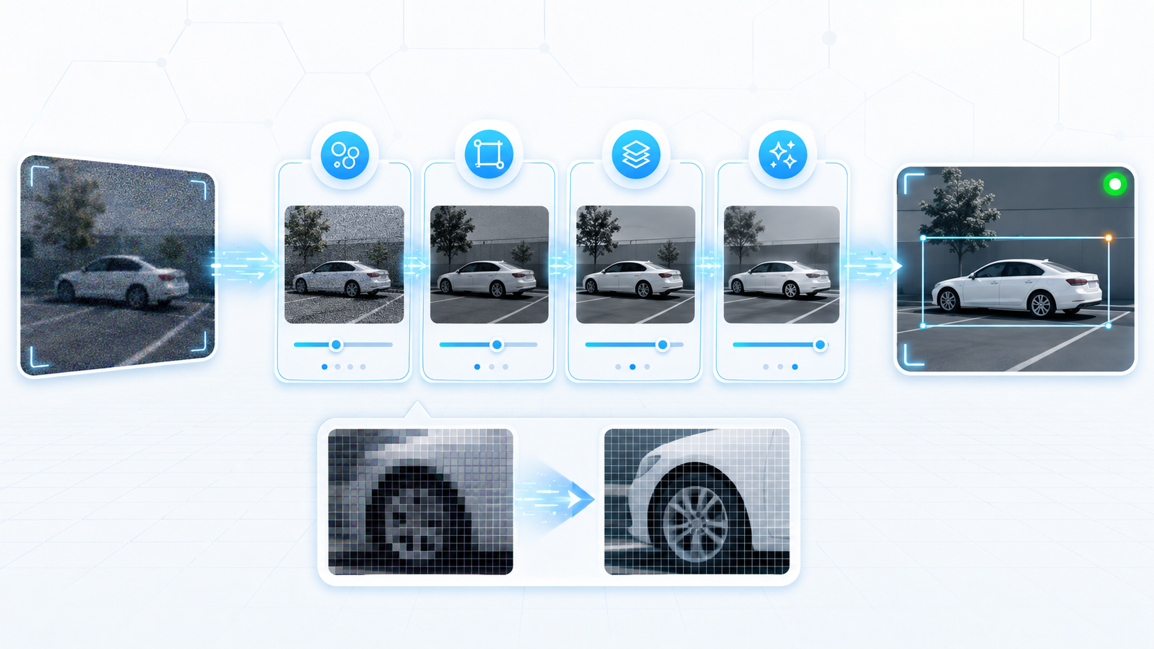
The model gets all the glory. In every demo video, every conference keynote, every breathless LinkedIn post, the star is the neural network: it spots the intruder, reads the license plate, counts the crowd. The model is the celebrity chef. Cameras flash, applause, the dish plated beautifully.

Nobody photographs the person who washed the lettuce.

That person is image processing, and here is the uncomfortable truth that this entire episode rests on: the chef is only as good as the prep. Hand a world-class chef a counter of muddy, unwashed, badly cut ingredients and you get a bad dish, no matter how many awards hang on the wall. Hand a world-class detection model a noisy, over-compressed, crooked, badly lit frame and you get a bad detection, no matter how many GPUs you throw at it. Garbage in, garbage out, a phrase we have now earned three episodes in a row.

Welcome back to the Intelligent Video Analytics series. Last time we ended on a promise: the pixels have arrived, now we make them useful. That is the whole job of today. We are going to follow a single frame from the moment it lands as raw light to the moment it is clean, framed, sliced, and plated, ready for the model to taste. So put on an apron. We are going into the kitchen.

Where we are: one step before the chef#

Remember the capture-to-storage chain from Episode 1? Scene, lens, sensor, processor, transmission, recorder, analytics. Episode 1 lived at the glass. Episode 2 lived in transmission and the recorder. Today we live in the narrow, busy, decisive strip right before “analytics,” and partly inside it: the processing that turns stored, delivered pixels into something a model can reason about.

Think of it as the prep station in a restaurant kitchen. The ingredients have been delivered (Episode 2). Now, before any cooking happens, someone has to wash them, trim them, portion them, and lay them out straight. Skip the prep and the most expensive chef in the world makes you a bad meal. Here is the full prep line we are going to walk:

flowchart LR
    RAW[Raw frame] --> ENH[Enhancement<br/>wash and sharpen]
    ENH --> CMP[Compression<br/>portion sensibly]
    CMP --> TRF[Transformation<br/>straighten and re-aim]
    TRF --> DET[Detection<br/>where is it?]
    DET --> SEG[Segmentation<br/>which exact pixels?]
    SEG --> AI[Analytics / the model]

We will take these in order, with one detour at the very start, because before you can wash an ingredient you have to know what it actually is. And a digital image, it turns out, is not a picture at all. It is a spreadsheet.

A picture is just numbers#

Here is the mental shift that makes the rest of this episode click. To a computer, an image is not a scene. It is a grid of numbers. Every “photo” is really a giant table where each cell holds a value describing how bright or what color one tiny patch of the world is. That tiny patch is a pixel (short for “picture element”).

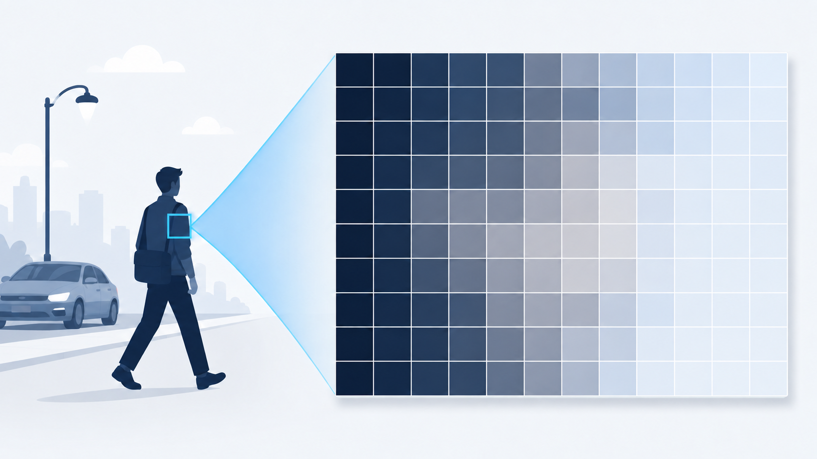
Zoom in far enough and the photograph disappears: every pixel is just one number describing how bright that patch of the world is. The whole episode rests on this flip from picture to spreadsheet.

Getting from real, continuous light to that neat grid of numbers takes three steps: scanning, sampling, and quantization. Let us take them one at a time.

Scanning is the camera systematically sweeping the scene and turning incoming light into an electrical signal. The lens focuses light onto an image sensor (CMOS in most modern cameras, as we met in Episode 1), and the sensor converts photons into a measurable voltage. At this point the signal is still continuous, a smooth analog wave.

Sampling chops that continuous image into a grid of discrete points: the pixels. How finely you chop is the resolution. A 1920×1080 (“Full HD”) frame is a grid 1920 pixels wide and 1080 tall, which is 2,073,600 pixels in total. An old 640×480 frame is only 307,200 pixels, which is why it looks blocky the moment you blow it up: there simply are not enough cells in the spreadsheet to describe the detail.

There is a tidy formula for how densely you are sampling, expressed as pixels per physical unit of the original scene:

A quick warning before the example: the word “sampling rate” here means spatial density (pixels per centimeter of scene), not the temporal frame rate (frames per second) we will talk about later. Same two words, very different meaning. The English language overloaded the term; do not let it trip you.

Worked example: you have an analog image measuring 4 cm by 3 cm, and you want to digitize it at 1024 x 768.

Horizontal sampling = 1024 px / 4 cm = 256 px/cm
Vertical   sampling =  768 px / 3 cm = 256 px/cm
Overall = 256 x 256 = 65,536 px/cm^2

So you are packing about 65,536 pixels into every square centimeter of the original scene. The higher that number, the finer the detail you capture. There is a ceiling, though, named after Harry Nyquist: to represent detail faithfully you must sample at least twice as finely as the smallest feature you care about. Sample too coarsely and you get aliasing, the digital gremlin that turns fine stripes into weird moire patterns and makes spinning wheels look like they rotate backwards. Sample finely enough and the gremlin stays in its box.

Quantization: turning brightness into a number, and the math behind it#

Sampling decided where the pixels are. Quantization decides what number each pixel holds. Because a computer cannot store an infinite range of brightness, it has to round each pixel’s intensity to one of a fixed set of levels. How many levels? That is the bit depth. An 8-bit grayscale image has 2^8 = 256 possible brightness levels, from 0 (pure black) to 255 (pure white). A 24-bit color image is just three of those 8-bit channels stacked: 8 bits for red, 8 for green, 8 for blue.

This is worth doing properly rather than hand-waving, so let us roll up our sleeves. It is not scary; it is one division and one rounding.

First you compute the step size, the gap between adjacent levels:

Then you map any real intensity to the nearest level below it and reconstruct the stored value:

The floor just means “round down to the nearest whole step.” That is the whole trick. Let us run a grayscale example: intensities range from Imin = 0 to Imax = 255, and we only allow L = 8 levels (a deliberately coarse setting to make the math visible).

Step 1  dI = (255 - 0) / 8 = 31.875
Step 2  for an actual intensity I = 100:
        Q = floor( (100 - 0) / 31.875 ) x 31.875 + 0
        Q = floor( 3.14 ) x 31.875
        Q = 3 x 31.875 = 95.625  ~  96

So a pixel that was really at brightness 100 gets stored as 96. The difference, 100 minus 96, is the quantization error: the small, unavoidable rounding mistake you make every time you force a smooth range into a finite set of steps. With only 8 levels the error is visible (you would see banding in a smooth sky). Crank L up to 256 (true 8-bit) and the steps get so fine, about 1 unit each, that your eye stops noticing. That is precisely why 8 bits per channel became the industry default: it is the sweet spot where the quantization error drops below human perception without wasting storage.

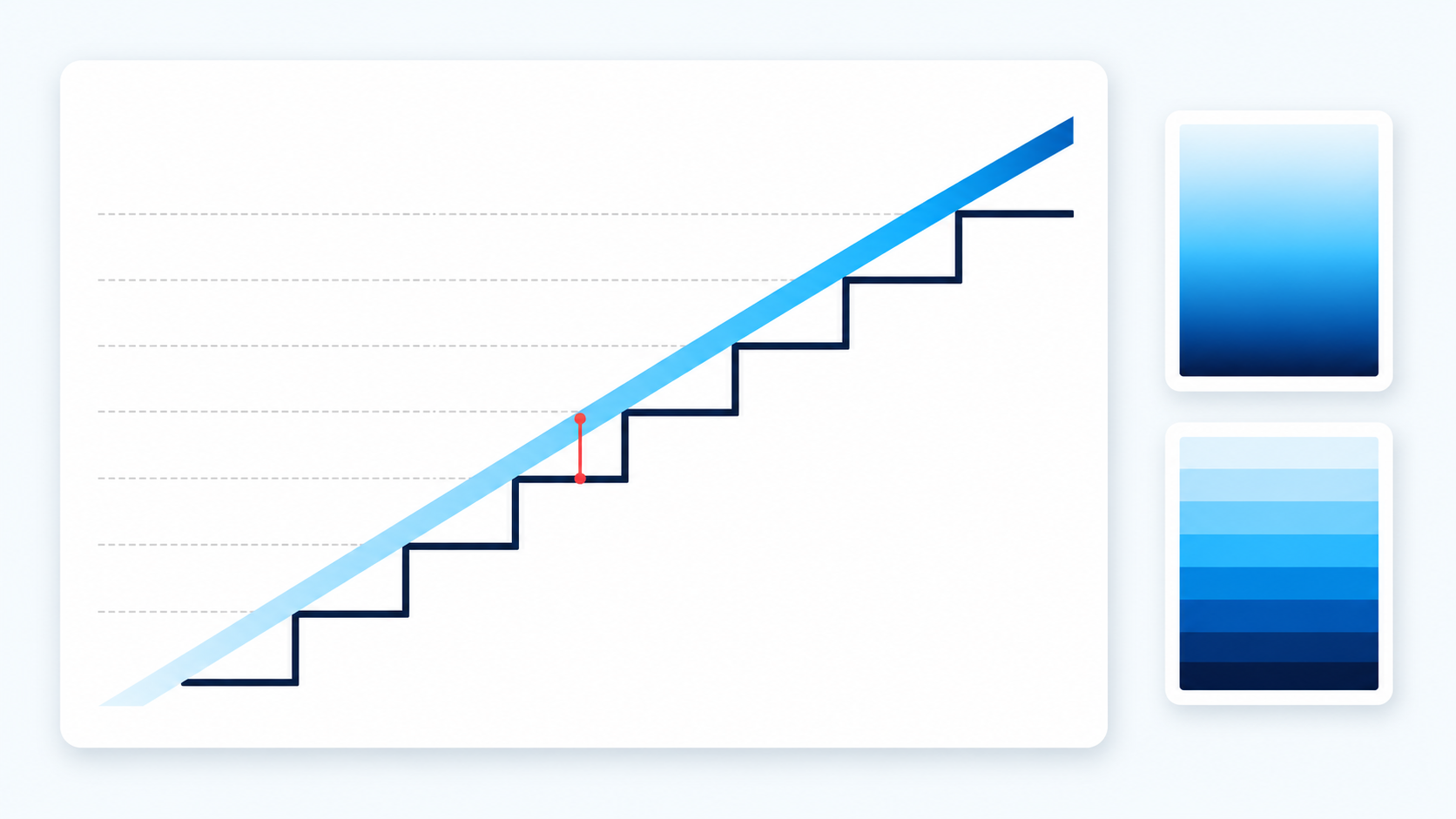
The cyan ramp is real, continuous brightness; the navy staircase is what 8 levels can actually store. The red gap is the quantization error: intensity 100 lands on rung 96. Raise the level count to 256 and the rungs get so fine the banding on the right vanishes.

Color works the same way, just three times over. Here is an RGB pixel quantized to L = 4 levels per channel:

dI = 255 / 4 = 63.75
Red   200 -> floor(200/63.75)=3 -> 3 x 63.75 = 191.25  ~ 191
Green 150 -> floor(150/63.75)=2 -> 2 x 63.75 = 127.5   ~ 128
Blue   50 -> floor(50/63.75) =0 -> 0 x 63.75 = 0
Result: (200,150,50) -> (191,128,0)

The original color shifts slightly because each channel got rounded to one of only four rungs. Use 256 rungs instead and the shift becomes invisible. The lesson generalizes: more bits means smaller steps means less rounding error means cleaner data for the model, traded against storage and bandwidth. It is the same fidelity-versus-cost tug-of-war we met with compression in Episode 2, just one layer deeper.

How we store the picture: image representations#

Now that a pixel is a number, the next question is how many numbers per pixel, and what they mean. Surveillance systems lean on four representations, and the smart move is matching the representation to the analytic task instead of always reaching for full color.

A binary image stores just one bit per pixel: 0 or 1, off or on. It is the simplest possible representation, useless for recognizing a face but perfect for a motion mask, where all you care about is “did this pixel change or not.” Background subtraction and intrusion-zone logic live here. Cheap and instant.

A grayscale image stores one 8-bit intensity (0 to 255) per pixel: brightness only, no color. This is the natural format for infrared (IR) and night-vision footage, and it is plenty for motion detection, object counting, and shadow analysis. Half the data of color, and for many tasks no real loss.

A color (RGB) image stores three 8-bit channels per pixel. This is the default diet for most AI models in surveillance, because color is a rich contextual cue: face recognition, “find the person in the red jacket” searches, and license plate reading all want it. Richness costs storage, but for recognition it usually earns its keep.

A multichannel (or multiband) image goes beyond three channels to include things like thermal, ultraviolet, or full hyperspectral bands (hundreds of wavelengths). Rare in everyday CCTV, but increasingly real in perimeter security and critical-infrastructure monitoring, where a thermal band can spot a person in pitch darkness that no RGB camera would ever see.

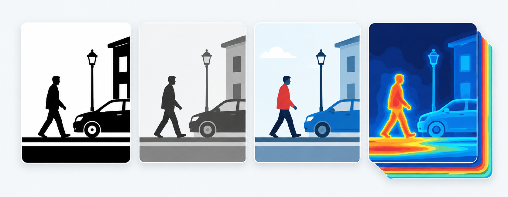
Left to right: binary (1 bit, enough for a motion mask), grayscale (8 bits, fine for counting and night IR), colour RGB (24 bits, what most recognition models want), and multichannel (thermal and beyond, for perimeter work in the dark). Richer is not better, it is just more expensive. Pick the lightest one that still does the job.

Two practical wrinkles worth knowing. First, IVA platforms often convert RGB internally into other color spaces like YUV (which separates brightness from color) or HSV (hue, saturation, value), because separating brightness from color makes detection more robust when the lighting keeps changing. Second, high-contrast scenes (think a glass lobby door with bright sun outside and shadow inside) need WDR (Wide Dynamic Range) to keep both the highlights and the shadows readable. True WDR captures multiple exposures in a single frame and merges them; digital WDR fakes it after capture with gamma correction and histogram stretching. Without WDR, the person walking in from the sunlight is just a silhouette, and a silhouette has no face for your model to recognize.

A neat real-world combo: a city command center runs grayscale sub-streams for cheap real-time motion analytics, keeps full-color high-resolution streams for identity verification, and layers a thermal band on top to catch intruders in dark industrial zones. Three representations, three jobs, one system.

flowchart LR
    L[Light] --> SC[Scanning<br/>light to signal]
    SC --> SA[Sampling<br/>signal to pixel grid]
    SA --> QZ[Quantization<br/>pixel to number]
    QZ --> G[(Digital image:<br/>a grid of numbers)]

That is the raw ingredient understood. Now we start prepping it. First job: wash it.

Enhancement: washing and sharpening the ingredients#

Real surveillance footage arrives dirty. Image enhancement is the set of techniques that clean it up, and here is the crucial difference from the photo app on your phone: enhancement for analytics is not about making the picture pretty for a human, it is about making the features clear for a machine. Nobody cares if the night-time parking lot looks moody and cinematic; they care whether the model can still find the license plate.

Footage fights five recurring enemies. Noise, the random speckle that creeps in from low light, cheap sensors, or heavy compression, smears fine detail and triggers false detections. Bad brightness, under- or over-exposure, hides subjects in crushed shadows or blown-out highlights. Blur, from poor focus or compression, softens the very edges a model needs. Lens and motion defects, like chromatic aberration or smearing on a fast-moving car, distort shapes. And geometric distortion from fisheye or wide-angle lenses warps the whole scene so a person near the edge looks bent.

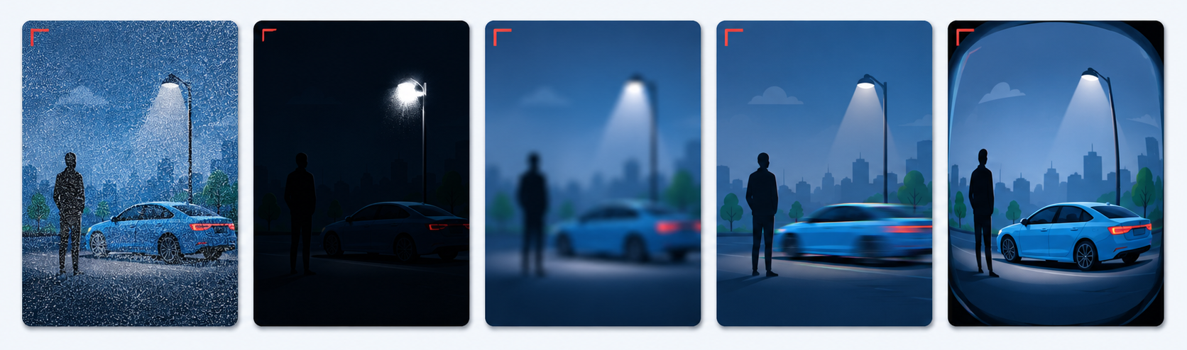
The same frame, five ways to be unusable: noise, bad brightness, blur, lens and motion defects, and geometric distortion. Enhancement exists to undo these before the model ever sees the frame, and each enemy has its own tool.

The tools to fight back split into two camps. Spatial-domain techniques work directly on the pixel numbers: contrast stretching pulls a dull, low-contrast image across the full 0-to-255 range; gamma correction brightens or darkens with a power-law curve; smoothing (a Gaussian or median filter) averages out random noise; and sharpening boosts edges. Frequency-domain techniques first transform the image into its frequency components (more on transforms shortly) and then tweak those: a high-pass filter emphasizes fine detail like plate text and facial landmarks, while a wavelet transform lets you enhance fine and coarse detail separately.

Sharpening is worth a one-formula detour, because it reveals what “an edge” even is to a computer. An edge is just a place where brightness changes fast. Measure how fast it changes in the x and y directions, combine them, and you get the edge gradient magnitude:

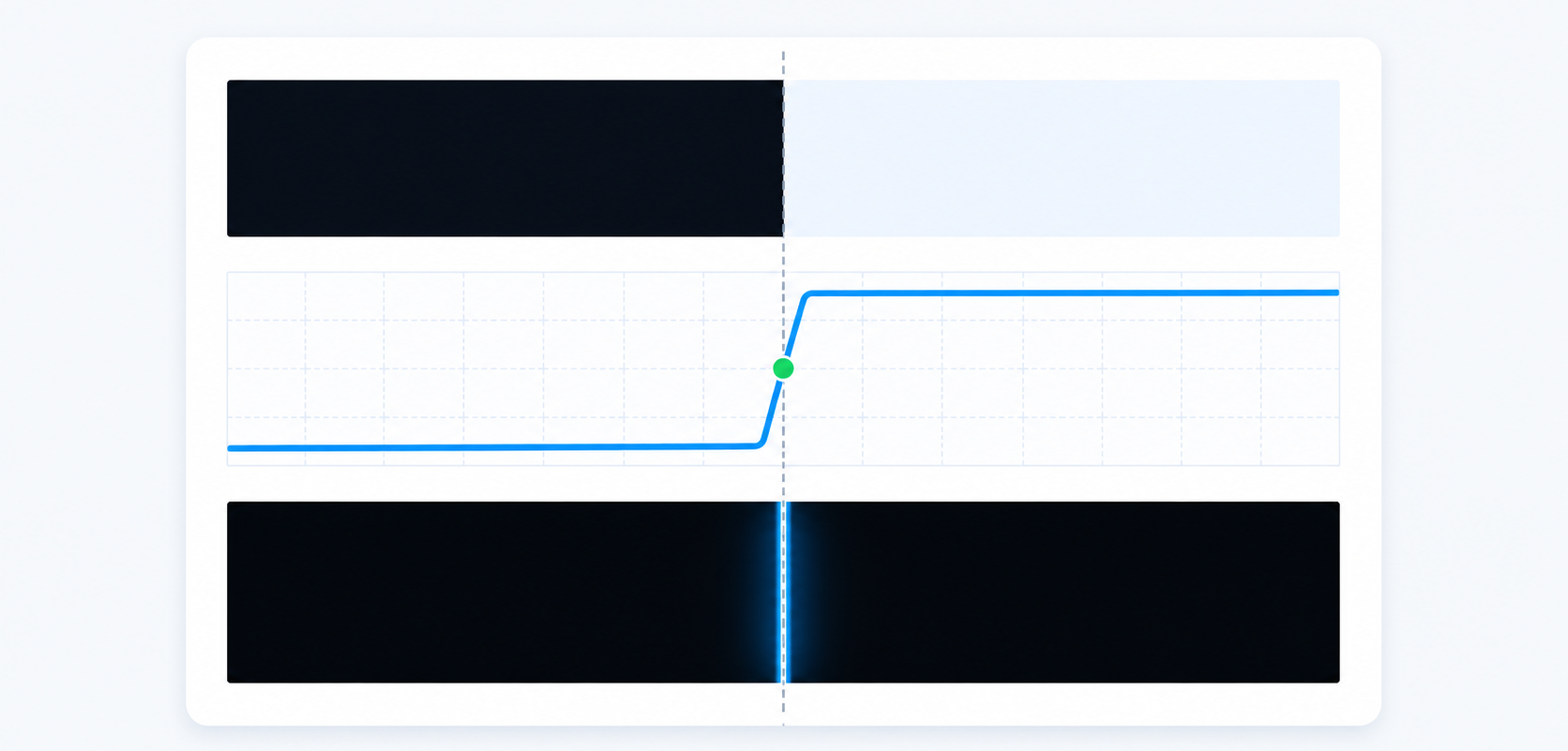
Top: brightness jumps from dark to light. Middle: the rate of change spikes at exactly that jump. Bottom: that spike is the edge. Big G means a strong boundary, small G means flat surface. Hold onto this, it is how neural networks start seeing in Episode 4.

Big G means a strong edge (the boundary of a car); small G means a flat region (the road surface). Sharpening filters like Laplacian, Sobel, and unsharp masking all amplify high-G regions, which is exactly why a sharpened frame helps shape-based detection. Hold onto this idea: it is the seed of how neural networks “see” in Episode 4.

Low light deserves its own line because it is where most outdoor systems quietly fail. The processing-side playbook: apply histogram equalization or adaptive contrast enhancement to claw back detail from the gloom; run spatial denoising (median or Gaussian) or temporal denoising across frames; combine motion deblurring with stabilization; and lean on IR-enhanced grayscale streams with a contrast boost. In a tunnel, that pipeline is the difference between a readable plate and an unreadable smear, captured on the exact same mid-range sensor.

Compression: portion control without starving the model#

Episode 2 taught us why we compress: raw video is comically huge and the network is finite. This episode is about how, and why doing it carelessly poisons the meal.

Compression works by removing three kinds of waste. Spatial redundancy is neighboring pixels that look almost the same (a big patch of blue sky barely needs to be described pixel by pixel). Psycho-visual redundancy is detail your eye cannot perceive anyway, so why spend bits on it. Coding redundancy is just inefficient bookkeeping, using more bits than a value needs. Squeeze out all three and the file shrinks dramatically.

There are two philosophies. Lossless compression (PNG, TIFF, GIF) preserves every original pixel value exactly; you use it in forensics or regulated settings where altering a single pixel is unacceptable. Lossy compression (JPEG, H.264, H.265, WebP, HEIF) throws away the least-important data to shrink files far more aggressively; it is the workhorse of live streaming and real-time analytics. A quick clarification, since the chapter mixes them: JPEG and PNG are still-image formats, while H.264 and H.265 are video codecs, but they all share the same underlying ideas.

The machinery that does the squeezing is a codec, a word welded together from coder and decoder. The encoder compresses, the decoder rebuilds. Encoding runs three steps: transformation converts the image from raw pixels into frequency components, usually with the Discrete Cosine Transform (DCT), which neatly separates the important low-frequency structure from the discardable high-frequency fuzz; quantization then rounds those frequency coefficients (yes, the same rounding idea from earlier, applied in frequency space) and throws away the insignificant ones; and entropy encoding (Huffman or arithmetic coding) packs the survivors using short codes for common values. Decoding simply runs all three in reverse: entropy decode, dequantize, inverse transform, and you have a viewable frame again.

flowchart LR
    IMG[Raw frame] --> T[Transform<br/>DCT / wavelet]
    T --> Q[Quantize<br/>drop fine detail]
    Q --> E[Entropy code<br/>Huffman / arithmetic]
    E --> BS[(Compressed<br/>bitstream)]
    BS --> ED[Entropy decode] --> DQ[Dequantize] --> IT[Inverse transform] --> OUT[Rebuilt frame]

Modern smart codecs (H.265, AV1) add a layer of intelligence that matters enormously for analytics. ROI (Region of Interest) encoding spends a high bitrate on the parts that carry meaning, the moving person, the license plate, the face, while aggressively compressing the static background. Scene-adaptive bitrate control dials compression up on quiet scenes (an empty hallway) and down on busy ones (a crowded intersection), automatically. And sub-streaming, which we met in Episode 2, emits a low-resolution stream for live viewing and a high-resolution one for the archive and analytics, from the same camera.

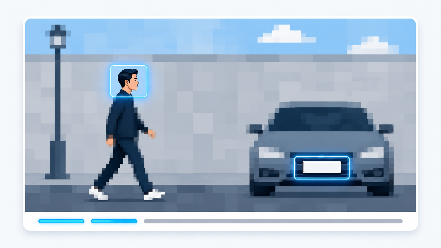
ROI encoding does not spend more bits, it spends them somewhere else. The face and the plate stay sharp; the empty wall gets crushed. Pixels on target, again.

When the input is already degraded, AI can play rescue. Super-resolution reconstructs plausible fine detail from a low-resolution stream, boosting a fuzzy face or plate. Frame interpolation invents intermediate frames for footage shot at a low frame rate, smoothing motion so trackers do not lose objects between jumps. Artifact suppression uses trained models to scrub out compression damage while protecting real edges. One honesty caveat, because forensics demands it: super-resolution and interpolation produce plausible detail, not recovered truth. They help a model, but a reconstructed plate is not courtroom-grade evidence. Useful prep, not magic.

The artifact caveat: the Episode 2 promise, paid off#

In Episode 2 I promised this moment would come back to bite, so here it is. Compression is lossy, and pushed too hard it does not just make footage uglier, it destroys the exact information your analytics depends on.

Left to right: healthy bitrate, then macroblocking with mosquito noise and ringing creeping in, then total collapse. Every one of these attacks edges, and edges are exactly what your detector reads. The plate did not get uglier, it stopped existing as information.

Transformation: straighten and re-aim the pixels#

Enhancement cleaned the ingredients. Compression portioned them. Transformation is the prep step where you straighten and re-aim them, because cameras almost never see the world from the convenient angle a model was trained on. Unlike enhancement (which changes how a pixel looks) or compression (which changes how it is stored), transformation changes where pixels sit and how the geometry is laid out.

Five families of transform do the work. Geometric transformations move pixels around without changing their values: translation shifts the frame (handy for stabilizing a jittery camera), rotation spins it (to normalize an overhead view), scaling resizes it (to unify resolution across feeds), and shearing skews it (rare, but it shows up in forensic matching). Affine and projective transformations are the heavy lifters: affine transforms preserve straight lines and parallels (great for aligning frames across cameras), while projective transforms correct perspective entirely, turning a slanted oblique view into a clean head-on one. Intensity transformations like histogram equalization remap brightness rather than position. Frequency and wavelet transformations convert pixels into frequency components for filtering and multi-scale feature extraction. And morphological transformations clean up binary or segmented images: dilation and erosion grow or shrink object shapes to remove speckle, while opening and closing tidy up blobs so an object reads as one solid thing instead of a scatter of fragments.

Why bother with any of this? Because four killer use cases depend on it. Multi-camera tracking and re-identification (Re-ID) hands the same person off between cameras, using geometric matching (homography) where views overlap and deep-learning appearance matching where they do not; without consistent geometry, “person 47” on camera A becomes a stranger on camera B. Bird’s Eye View (BEV) reconstruction warps an angled camera into a top-down map, which is what makes crowd-density heatmaps and clean vehicle-flow analysis possible. Camera calibration and rectification undoes lens distortion (the barrel and fisheye bending from Episode 1) so straight real-world lines stay straight in the image, which is essential for accurate distance estimation. And perspective warping normalizes oblique hallway or entrance views into a consistent frontal or top-down shape so an object is the same size and orientation wherever it appears.

A tidy example: in a mall, security applies a projective transformation to convert oblique ceiling-camera angles into top-down maps, which makes real-time people counting and heatmap generation suddenly straightforward. The crooked view became a flat map, and a flat map is something you can actually measure.

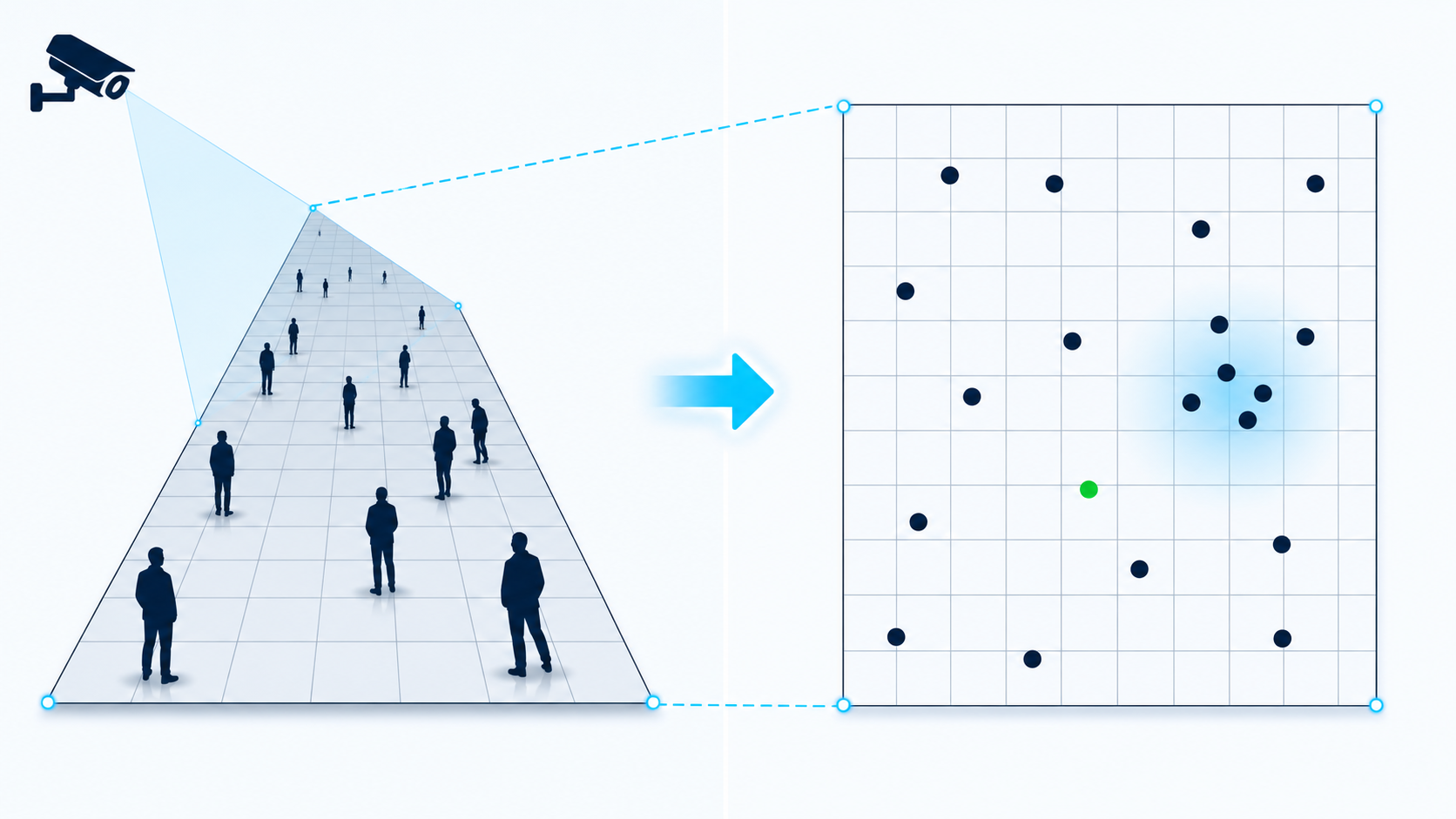
A projective transformation maps the four corners of the crooked view onto a flat rectangle. People who were different sizes because they stood further away become dots of equal weight, and only then can you honestly count them or draw a density heatmap.

Detection: where is the thing?#

Now the prep is done and we take the first real bite of seeing. The first question any analytic asks is simple: where is the thing, and what is it? That is object detection, and it is worth separating clearly from its cousin, classification. Classification labels a whole frame (“this image contains a car”). Detection goes further: it draws a bounding box around each object and labels it (“a car, here; a person, there; a bag, over there”), outputting coordinates plus a class label plus a confidence score for every object it finds. Those boxes are what downstream tracking, counting, and rule-violation alerts feed on.

Three deep-learning detectors dominate, and the trade-off between them is always speed versus accuracy. YOLO (You Only Look Once) processes the whole frame in a single pass, which makes it fast and the favorite for edge devices and real-time work. SSD (Single Shot Detector) predicts boxes from feature maps at multiple scales, striking a middle balance. Faster R-CNN is the most accurate and the heaviest, using a region-proposal network, so it suits forensic or high-end analytics where you can spend the compute.

To see how detection actually works under the hood, it helps to walk through the classic R-CNN pipeline in four steps, because it is genuinely intuitive:

1. Input image. Start with a frame containing objects of interest, say a person on a horse.
2. Extract region proposals. Rather than examine the whole image at once, the algorithm proposes roughly 2,000 candidate boxes (“something might be here”) using a technique like Selective Search, narrowing the search space.
3. Compute CNN features. Each proposed region is resized to a fixed size and pushed through a Convolutional Neural Network, which extracts features: edges, textures, patterns. (Remember the edge gradient from the enhancement section? This is that idea, learned and stacked.)
4. Classify regions. A classifier labels each region (“person,” “car,” “nothing”) and refines the box. Here it correctly tags the person and rejects the clutter.

And here is the link to that edge gradient I told you to hold onto. A CNN finds features by sliding a small filter across the image and computing, at each spot, a weighted sum of the pixels under it. That operation is convolution:

In plain words: I is the image, K is a little kernel (a feature detector), and you slide K over I to light up wherever that feature appears. One kernel might fire on vertical edges, another on a particular texture. Stack thousands of them across many layers and you get a model that learns to recognize a face. The detector then tunes its boxes by minimizing a bounding-box regression loss, essentially the summed squared error between its predicted box corners and the ground-truth corners, nudging the boxes until they hug the objects. We will not dwell on that formula; just know “the model is literally being scored on how tightly its boxes fit, and it trains to lower that score.”

Segmentation: which exact pixels?#

Detection drew a box. But a box around a person still contains a lot of not-person: background between the arms, a sliver of the wall, the floor under the feet. Image segmentation goes one level finer and labels every single pixel: this pixel is person, this pixel is road, this pixel is background. Where detection says “a person is roughly here,” segmentation traces the exact silhouette. It is the difference between circling someone in a photo and carefully cutting them out with scissors.

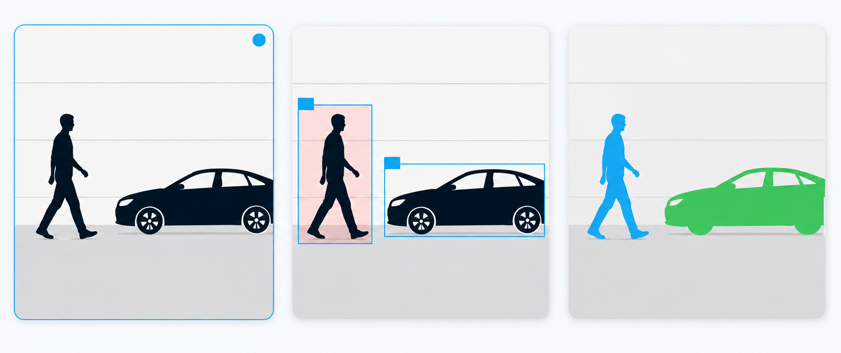
Classification labels the frame, detection boxes the objects, segmentation cuts them out. The red wash in the middle panel is everything a bounding box gets wrong: wall, floor, and the gap between the arms all counted as “person”.

That precision unlocks things a box cannot. People masking isolates a person’s exact shape for pose analysis or privacy blurring. Vehicle segmentation separates a car from the road so the plate region is clean. Crowd and queue detection measures real density and queue length by counting actual occupied pixels, not overlapping boxes. And intrusion detection can fire only when genuine foreground pixels cross a boundary, cutting false alarms from shadows and headlights.

Classic threshold-based methods have largely given way to deep learning here. The Fully Convolutional Network (FCN) was the first architecture built for pixel-wise labeling. U-Net, with its encoder-decoder shape, is beloved because it works well even with small training datasets, which is why it crosses over from medical imaging into surveillance. DeepLabV3+ uses clever multi-scale tricks (atrous convolutions and spatial pyramid pooling) to handle busy outdoor scenes. And the newest wave, Vision Transformers (ViTs) and Meta’s Segment Anything Model (SAM), use attention to segment almost anything, often from a simple prompt, which is a genuine leap in flexibility.

Raw masks are rarely perfect, so a post-processing pass tidies them: Conditional Random Fields (CRFs) sharpen boundaries, graph cuts and morphological operators (our friends dilation and erosion again) clean stray edges, and feature embeddings from the mask can even be used to re-identify the object across cameras. One closing example ties the whole episode together: in a mall, an IVA system uses SAM or U-Net to segment each customer at the entrance, feeds those clean masks into a Re-ID pipeline that follows the same person across non-overlapping cameras (ignoring mannequins and reflections), and simultaneously compares foreground maps over time to flag a bag left behind near the seating. Segmentation, transformation, and detection all cooperating, each one prepped by the steps before it.

Putting it together: from raw counter to plated dish#

Step back and look at the whole kitchen. A frame lands as raw light and becomes a grid of numbers (sampling and quantization). We pick the right representation for the job (grayscale for cheap motion, RGB for recognition, thermal for the dark). We wash it (enhancement), portion it without starving the model (compression, with ROI keeping the bits where they matter), and straighten it (transformation) so the geometry makes sense. Then come the first acts of understanding: detection draws the boxes, segmentation cuts the exact shapes, and only then does the model in the analytics block get a clean, well-organized plate to reason about.

In a real metro station, that full line runs continuously: enhancement claws detail out of dim platform footage, smart compression keeps 400 feeds on the network, transformation hands a commuter off between platform cameras, detection flags a person loitering in a restricted zone, and segmentation isolates an unattended bag by comparing foreground over time. None of it is the “AI” everyone photographs. All of it is the prep that makes the AI possible.

The “is my footage prepped?” checklist#

Mirroring the camera checklist from Episode 1 and the network checklist from Episode 2, here is the prep-station gut-check. If you cannot answer yes to these, the chef is going to struggle no matter how good they are.

1. Resolution and bit depth: is the footage sampled finely enough and quantized deeply enough (8-bit minimum per channel) to carry the detail the task needs?
2. Representation fit: am I using the lightest representation that still works (grayscale for motion, RGB for recognition, thermal where it earns its place)?
3. Enhancement: are noise, brightness, blur, and lens distortion handled before the frame hits the model, especially in low light?
4. Compression discipline: is the codec efficient (H.265 where hardware allows) and the bitrate high enough on the regions that matter (ROI encoding) to avoid artifacts in critical zones?
5. Geometry: are oblique or distorted views rectified and, where needed, warped to a consistent perspective for counting and tracking?
6. Detection readiness: are the edges and contrast strong enough that a detector can actually find and box objects?
7. Segmentation and post-processing: where per-pixel precision matters, is the mask cleaned (CRF, morphology) before downstream use?
8. Honesty about rescue tools: am I treating super-resolution and interpolation as helpful prep, not as recovered ground truth?

Wrapping up#

Image processing is the prep cook of video analytics: unglamorous, rarely photographed, and completely decisive. We turned light into numbers and did the real quantization math, learned which representation to reach for, washed footage clean with enhancement, portioned it with compression while dodging the artifacts that wreck detection, straightened it with transformation, and took the first true bites of seeing with detection and segmentation.

The short version, if you forget everything else: a model is only as good as the frame you hand it, so clean it, frame it, slice it, and plate it before you let the AI taste it.

Next episode, the celebrity chef finally walks into the kitchen. Episode 4 is deep learning for vision: neurons, convolutional neural networks, transfer learning, and how all those features we kept hinting at actually get learned. We have prepped the ingredients beautifully. Now we cook. See you there.