Building Your First Neuron From Scratch

This is Part 2 of the Deep Learning Foundations series. In Part 1 we built a mental model: machine learning learns rules from examples, deep learning learns them in layers, and training is a loop that measures error and nudges weights downhill. We deliberately stayed abstract. Now we open the hood.

Here is the promise from last time, made concrete. The smallest working piece of a neural network is a single neuron, and it genuinely fits on a napkin. It takes a few numbers in, multiplies each by a weight, adds them up, and decides yes or no. Training it is a three-line loop. Let’s build it in NumPy, from scratch, no framework, and watch it learn to separate blue dots from white ones. Once you have felt a handful of numbers learn on your own screen, deep learning stops being mysterious for good.

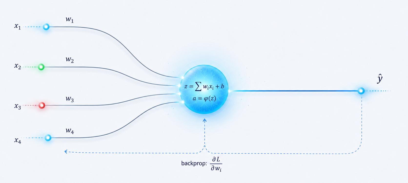
The smallest working unit of a neural network. A few inputs come in, each scaled by how much the neuron trusts it, and one decision comes out. Everything else in deep learning is many of these, wired together.

What an artificial neuron actually is#

The artificial neuron borrows its name, and only loosely its shape, from biology. A brain cell fires an electrical signal when the combined input from its neighbors crosses some threshold. The artificial version keeps that one idea, a unit that combines several inputs and then decides whether to fire, and throws away everything else. As we stressed in Part 1, this is inspiration, not a model of the brain. Do not read too much into the word “neuron.”

Mechanically, a neuron does three tiny things. It takes a vector of inputs x. It computes a weighted sum of them, where each weight says how much that input matters, and adds a bias term b that shifts the result. Then it passes that sum through an activation function that produces the output. The weighted sum is worth naming; we will call it the activation potential:

p = w · x + b

Here w · x is the dot product, w[0]*x[0] + w[1]*x[1] + ..., and b is a single number that lets the neuron lean toward firing or not firing before it has seen any input at all. Think of the neuron as a tiny voting machine: the weights are how much it trusts each input, the bias is its baseline lean, and the activation function is how decisively it turns that tally into a yes or a no.

flowchart LR
    X0["x₀"] --> S
    X1["x₁"] --> S
    X2["x₂"] --> S
    B["bias b"] --> S
    S["Σ weighted sum<br/>p = w · x + b"] --> A["activation<br/>f(p)"]
    A --> Y["output y"]

An artificial neuron. Each input is scaled by a weight and summed with the bias to give the activation potential p, which the activation function turns into the output.

In NumPy that is almost nothing:

import numpy as np

def neuron(w, b, x):
    p = np.dot(w, x) + b     # activation potential
    return step(p)           # activation function -> output

We just need to decide what step is.

The simplest activation: fire or don’t#

The most basic activation is the Heaviside step function. It outputs 1 if the potential is positive and 0 otherwise. Fire, or stay quiet.

def step(p):
    return (p > 0).astype(int)

A neuron with a step activation is a binary classifier: give it an input and it answers class 1 or class 0. Right now its weights are random, so its answers are random too. To make it useful, we have to train it.

Training it: nudge on error#

Here is the whole training idea, and it is the same loop from Part 1 wearing work clothes. Show the neuron one example, compare its guess to the correct answer, and if it got it wrong, shove the weights a little in the direction that would have helped. Do that thousands of times.

The rule for the shove is beautifully simple. Let y be the neuron’s prediction and t the true target. The error is just their difference, y - t, which for our binary case is always +1, 0, or -1. When the error is zero the neuron was right and we change nothing. Otherwise we update:

w  ->  w - η (y - t) x
b  ->  b - η (y - t)

The number η (the Greek letter eta) is the learning rate, a small value between 0 and 1 that controls how big each nudge is. That is it. That is the learning. In code:

rng = np.random.default_rng()
w = rng.standard_normal(2)   # two inputs -> two weights
b = rng.standard_normal()
eta = 0.1                    # learning rate

for _ in range(2000):
    i = rng.integers(len(X))         # pick a random example
    y = neuron(w, b, X[i])           # what the neuron guesses
    error = y - t[i]                 # +1, 0, or -1
    w = w - eta * error * X[i]       # nudge the weights
    b = b - eta * error              # nudge the bias

Run that loop and something quietly remarkable happens: the weights drift from noise into values that classify the points correctly, and they stay there. Nobody told the neuron the rule. It found it from the errors alone. This tiny block is the ancestor of every training loop in modern AI. Everything else is scale and refinement.

flowchart LR
    P["pick an example x"] --> G["neuron guesses y"]
    G --> E["error = y - t"]
    E --> U["nudge w and b<br/>by η · error · x"]
    U --> P

The from-scratch training loop. It is Part 1’s predict, measure error, adjust the weights, exactly, now in three lines of NumPy.

Two inputs, and a line that moves#

With two inputs, we can see what the neuron is really doing. Its decision depends on the sign of w[0]*x[0] + w[1]*x[1] + b. The set of points where that sum is exactly zero is a straight line, and the neuron says “class 1” on one side of it and “class 0” on the other. Training moves that line until it separates the two clouds of points. The weights set the line’s angle; the bias slides it away from the origin.

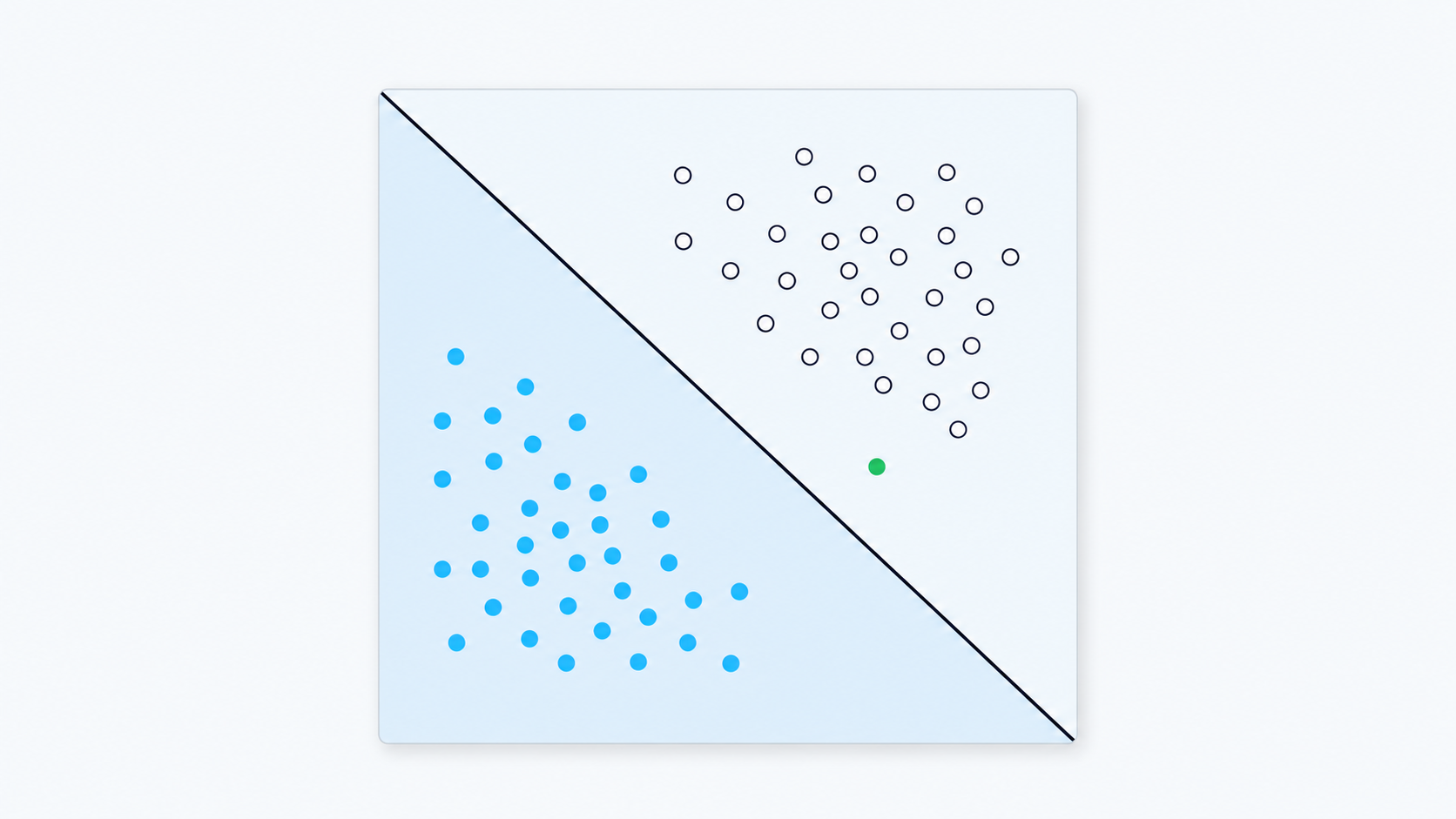
A trained two-input neuron draws a straight decision boundary. The weights tilt the line, the bias shifts it. Everything on one side is called class 1, everything on the other class 0.

That picture is the key to the neuron’s power and, as we are about to see, its hard limit. A single neuron can only ever draw one straight line.

A menu of activations#

The step function is honest but blunt: it only ever says 0 or 1, and it has a hard corner that makes it useless for the gradient-based training we will meet in Part 3. So in practice we swap it for a smoother activation. The common ones are worth recognizing:

The sigmoid squashes any input into a smooth S-curve between 0 and 1, which reads naturally as a probability. Tanh is its cousin, squashing into the range -1 to 1. The linear activation does nothing at all, returning the input unchanged, which is what you want when a neuron should predict a number rather than a class. The ReLU (rectified linear unit) passes positive values straight through and clamps negatives to zero; it is cheap to compute and dominates modern networks. Leaky ReLU is the same but lets a small trickle through for negatives, which helps training stay healthy.

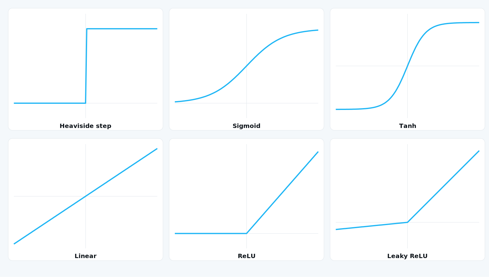
The common activation functions. The smooth ones (sigmoid, tanh, ReLU and friends) are continuous and differentiable, which is exactly what the training algorithm in Part 3 needs, and they let a neuron do regression as well as classification.

Two properties matter about the smooth activations. First, they are continuous, so a neuron can output a real number and tackle regression, not just yes/no classification. Second, they are differentiable almost everywhere, which is the property that makes backpropagation possible. Hold that thought; it is the whole subject of Part 3.

But swapping the activation does not change the neuron’s fundamental limit. It still computes a weighted sum and then a simple squashing, so its decision boundary is still a single straight line. To break past a straight line, we need more than one neuron.

The wall: one neuron draws one line#

Here is the classic problem that stopped early neural network research cold. Consider the exclusive-or, or XOR, pattern: two inputs, and the answer is 1 when exactly one of them is 1. Plot the four cases and the two classes sit on opposite corners of a square. No straight line can separate them. Try to draw one and you will always get a point wrong.

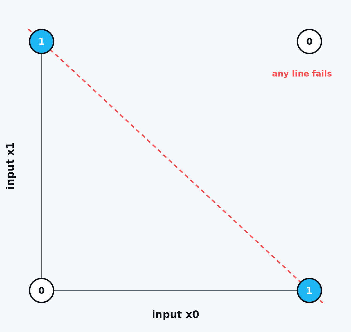
The XOR problem. The two classes sit on opposite corners, so no single straight line can split them. A single neuron, which can only draw one line, is stuck here.

A single neuron can happily learn AND, OR, and NAND, because each of those is separable by one line. It can never learn XOR. When this was pointed out in 1969, by Marvin Minsky and Seymour Papert, it helped freeze funding for neural networks for years, one of the AI winters we mentioned in Part 1. The fix turned out to be almost embarrassingly simple, but it took a while to become obvious.

Stacking neurons into a layer#

The fix is to stop using one neuron and use a small team of them, arranged in layers. Put two or three neurons in a first layer, each drawing its own line and carving the plane into half-planes. Then feed their outputs into a second neuron whose job is to combine those half-planes into a more complex region. Suddenly you can carve out shapes no single line could, and XOR falls immediately.

flowchart LR
    X0["x₀"] --> H0["neuron"]
    X1["x₁"] --> H0
    X0 --> H1["neuron"]
    X1 --> H1
    H0 --> O["output<br/>neuron"]
    H1 --> O
    O --> Y["y"]
    subgraph HID["hidden layer"]
        H0
        H1
    end

A two-layer network. The hidden layer’s neurons each draw a line, and the output neuron combines their results into a region a single line could never describe. This is a dense, or fully connected, network, also called a multilayer perceptron.

This arrangement has a few names you will see everywhere: a dense network, a fully connected network, or a multilayer perceptron (MLP). “Dense” because every neuron in a layer connects to every neuron in the next. The layer between input and output is called a hidden layer, and the number of layers is the network’s depth, exactly the “deep” from Part 1. With smooth activations, the whole two-layer network is just a short stack of the same weighted-sum-then-squash operation:

def dnn2(Wa, Wb, x):
    h = sigmoid(x @ Wa)     # hidden layer
    return sigmoid(h @ Wb)  # output layer

Add more hidden layers and the network can carve ever more intricate regions, classifying shapes that two layers cannot. That is the ladder we will keep climbing in this series, all the way up to a network that reads handwritten digits.

Wrapping up#

You just built a neural network’s smallest piece and trained it with arithmetic you could redo by hand. A neuron is a weighted sum of its inputs plus a bias, passed through an activation function. Training is a loop: guess, measure the error, and nudge the weights and bias by the error times a small learning rate. One neuron draws one straight line, which is enough for simple problems and useless for XOR. Stack neurons into layers and the straight-line limit disappears, at the cost of needing a smarter way to assign blame for errors. That smarter way is backpropagation, and it is next.

The short version: a neuron is activation(w · x + b); you train it by nudging w and b in proportion to its error; one neuron is a single line, and stacking them into layers is what lets a network learn anything more interesting.

What’s next#

In Part 3, we earn the one piece we hand-waved here. We will open up gradient descent and backpropagation: what a gradient actually is, why the smooth activations from this article matter, and how a network figures out which direction to nudge every weight, even the ones deep in the middle. It is the math that makes the “nudge on error” rule work for a network of any depth, and it is more intuitive than its reputation suggests. Bring the neuron you just built; we are about to teach a whole network of them to learn together.